What we built
We developed manipulator models across three levels of complexity: a cylindrical PRP workspace, a six-axis Stanford arm, and a planar 3R arm with dynamics and control. The sequence shows how the same frame discipline can progress from reachable geometry and pose calculations to symbolic dynamics, computed-torque control, waypoint motion, disturbance response, and Cartesian tasks.
SYSTEM ARCHITECTURE
Map a reachable workspace
PRP joint limits → homogeneous pose → work envelopeThe cylindrical robot connected joint limits to a visible three-dimensional workspace, including the inner region its radial joint could not reach.
Solve six-axis pose kinematics
six joint values ↔ end-effector position and orientationThe Stanford-arm model reused six frame transformations for forward pose, Cartesian and spherical inverse position, and wrist orientation.
Add dynamics and control
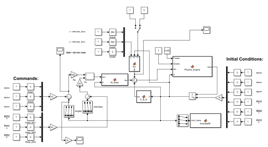
desired motion → computed torque → 3R physics model → animationSymbolic MATLAB produced the mass, Coriolis, and gravity terms for the planar arm. Simulink combined them with feedback to control joint commands, paths, disturbances, and Cartesian motion.
How the studies progressed
- STAGE 01
Map the cylindrical workspace
Swept the cylindrical robot's joint limits to visualize its reachable volume and added Cartesian inverse positioning.
- STAGE 02
Build Stanford forward and inverse kinematics
Built the Stanford arm's six-transform chain, then extended it from forward pose to inverse position and wrist orientation.
- STAGE 03
Derive the 3R dynamics
Derived the planar 3R transform, Jacobian, mass matrix, Coriolis terms, and gravity vector symbolically.
- STAGE 04
Control motion in joint and task space
Closed a computed-torque loop around the physics model, tuned its response, and exercised five tasks spanning pose hold, joint commands, spline paths, disturbances, and Cartesian motion.
Key engineering decisions
Keeping every coordinate frame consistent
A sign or axis error could appear as a distorted workspace, a flipped wrist, or incorrect gravity torque. Known-pose animations provided an immediate check on the transformation chain.
Moving from forward pose to inverse motion
Forward kinematics gives one pose for a joint vector, while inverse problems can have multiple or singular solutions. The 3R Cartesian controller mapped task-space error through the inverse Jacobian and therefore depended on staying away from singular configurations.
Tuning the model without overclaiming it
Increasing the feedback gains removed the earlier oscillation and produced an approximately one-second joint response in simulation. That demonstrates the controller structure, not a hardware-ready servo design.
What worked
- Workspace plots show the cylindrical robot's complete reachable volume and its inner dead zone.
- Stanford-arm animations demonstrate forward pose, inverse position, and wrist-orientation calculations on a six-axis model.
- The 3R report preserves the DH model, symbolic dynamics, computed-torque architecture, and controller tuning calculations.
- Plots and videos show pose hold, joint tracking, a five-waypoint spline, disturbance handling, and Cartesian commands in simulation.
What we took from it
A disciplined frame convention made the same transformation logic reusable across workspace analysis, six-axis pose calculations, and 3R dynamics.
Moving from joint regulation to Cartesian control exposed issues—especially singularities and solution ambiguity—that simple pose calculations could hide.
Animation is a strong sanity check, but numerical residuals and physical testing would be needed to validate performance beyond simulation.